Kaggle LISH MOA Update

Hacking Away

Recap: A fellow Metis alum suggested that we enter a Kaggle competition. This project on the Method of Action of pharmeceuticals is definitely a rich sandbox to try different forms of feature processing and neural network architectures.

PCA and Clustering

Review: EDA

The input rows (one per experiment, presumably) are just labeled with a cryptic “sig_id” (presumably concealing proprietary drug chemistry…not something geochemists worry a whole lot about). The experiments are labeled to indicate whether they are experimental or control, the treatment time (24, 48, 72 hours), and a dosage flag (D1 or D2, not much help there).

The meat of the data consists of 772 columns of gene expression measurements (labeled g-0 to g-771) and 100 columns of cell viability measurements (c-0 to c-99… no clues there!). Whatever these measurements actually are, they have all been scaled from -10 to +10 (at most). If you’re curious, I’ve plotted some distributions here.

The targets are a list of 206 Methods of Action (hence the name!) that are labeled 0 or 1 for whether that treatment acted in that manner or not. For example, did the drug candidate act as a calcium channel blocker? A chelating agent? A cannabinoid receptor antagonist, perchance?

PCA

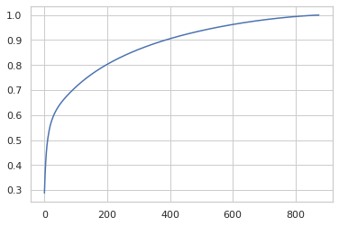
I’ve now tried a handful of strategies for preprocessing, combining feature encoding and scaling, PCA, and clustering. I’m discovering experimentally things like the dependence of PCA on the scales of the input features. In this case, if I leave treatment time at its raw values, they dominate the PCA breakdown. If, instead, I MinMaxScale them to -0.5 to 0.5 and StandardScale the gene and viability features, the PCA breakdown spreads the variation out like so:

MeanShift

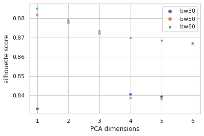
I lifted the idea of performing a clustering analysis on the data and using that as an additional set of categorical features from this notebook. Then I ran off in my own direction with it. I explored KMeans, DBSCAN, and MeanShift with varying k (1 to 10), in varying numbers of PCA dimensions (1 to 6) and it sure looked like MeanShift was at least giving the best silhouette scores, by a considerable margin in most cases. I dug down and considered the effects of setting the bandwidth at different quantiles (0.3 / 30%, 0.5 / 50%, 0.8 / 80%) for MeanShift:

How many clusters is that?

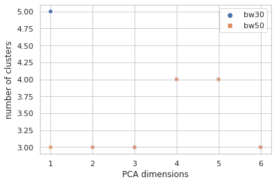
Sure seems worth the score hit to get five clusters of info with instead of four, so I went with the narrow bandwidth and… clustering in just the first PCA dimension? It looks a little quirky. Here I’m plotting the first two PCA dimensions and showing the clustering.

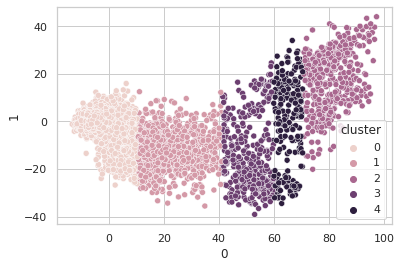
Obviously, clustering in 1-D, then plotting in 2-D, the clusters look like vertical bands. I hot encoded the cluster numbers, standard scaled the first 30 PCA dimensions, fed that to a neural network, and did indeed get a healthy bump in score once my kerastuner ground to a halt: from an uncompetitive 0.028 to a still-uncompetitive but lower 0.024. (Competitive, i.e. at least a bronze, would be below 0.0183, last I checked, and 0.01800 was just out of first place.)

Talking things over with my friend Matt, we decided to remove at least one redundant-seeming feature scaling step. I tried skipping the StandardScaling on the gene and cell features at the beginning, leaving them in the range -10 to 10 (while still MinMaxScaling the treatment times to -0.5 to 0.5 and encoding the treatment type and dose with 0 and 1), doing a PCA analysis on that, then clustering (five clusters in five PCA dimensions this time) and standard scaling these new PCA dimensions and taking 83 of them instead of 30–I have a really bad habit of trying too many things at once, but it takes Kaggle forever to grind through these notebooks and it’s hard to limit myself to one change each–when the dust had settled, I now had a score of 0.022.

Don’t get me started on trying to customize the loss function to match the competition. I’ll probably have to go back and pick that up on my own later. There are too many more interesting things to try.

–PAG

Blogging platform assembled by Jekyll, Poole, and Zach Miller of Metis.

Deep Learning on Nuclear Magnetic Resonance

ML4Sci

I left the last blog half an hour before a Machine Learning for Science event started. There were six events, and while I was tempted by the Google Earth competition, I really had to focus on the chemistry / solid state physics of the NMR event.

A Nickel of EDA

Basically, the goal was to go from simulated experimental data:

to four material properties (alpha, xi, p, and d):

Wading In

GitHub repo for this project

I took a broad approach. I really wanted to look at this data from a variety of angles, and that led me to automated machine learning (AutoML). As chronicled in my GitHub repo, I first attacked the problem with autosklearn, figuring that probably did not have the juice to really address the problem, but curious to find out what methods it would churn out as the best. It wound up being fairly hard to install, did not do as good as job as I’d hoped automating the preprocessing of data (it seemed to insist on treating continuous input values as categorical) and the results were really volatile, with adaboost, random forests, the “passive aggressive” regressor, and KNN methods all sometimes coming to the top. And the fits were bad. Still, it’s a tool I now know something about how to use for new problems.

Next I found AutoKeras, which is a little easier to install and a little better documented, for my purposes. It has the advantage of automating a search through some fairly high level options for setting up a Keras network. It, too, seems unable to believe I’d feed it straight numeric data and insisted on patching in some categorization tools. In any case, it got me started.

From there I moved on to kerastuner, which got me to reasonable models. Keras Tuner takes a structured description of a neural network and checks a manually designated set of options for things like layer width, activation function, learning rate, nearly all the hyperparameters of a neural network model. I ended up with my best scores (lowest weighted MSE losses) for a simple model with 900 input nodes to hold real and imaginary magnetization values at 450 time points and two hidden layers with 512 and 256 nodes to predict the 4 material properties. As you can see, the variables trained very differently:

Alpha trains up very well; p trains ok, and varies with hyperparameter choice and training duration. Xi is can’t train won’t train; I would need to dig into the theory to find out more. d is maddening. Basically, it’s a decay factor, and it seems as if it’s predictable up to a value of about 4, and after that the length of the experiment is apparently wrong for the purpose of clarifying it. It looks like a bloody logarithmic curve in the real vs. predicted plots, and I tried applying transforms to change it, but I think that’s trying to apply a bandage to a problem that needs to be addressed earlier in the process somehow; again, digging into the theory of what’s going on would be essential.

I tried regressing d by itself and using mean absolute error instead of a mean squared error metric, hoping for a plot where d lined up with predictions from 3 to 4 and then just flared out after that, which would be more sensible if I’m right about its behavior and its causes, but it didn’t look that different. Maddening. It’s one thing to jack around with the knobs and get unpredictable changes, but when no matter what you do to the knob you get the same problem, it’s frustrating.

–PAG

Blogging platform assembled by Jekyll, Poole, and Zach Miller of Metis.